Human Activity Recognition Using Smartphones

Introduction
Human activity recognition is the intresting problem of classifying sequences of accelerometer data recorded by smart phones into known well-defined movements.
It is a challenging problem given the large number of observations produced each second, the temporal nature of the observations, and the lack of a clear way to relate accelerometer data to known movements.
The difficulty is that this feature engineering requires deep expertise in the field. I would like to explore without bein an expert in sensor and tracking how well we can solve this problem.
After completing the business case, you will learn:
- How to load unseen human activity recognition data?
- How to explore the data using simple stats and t-SNE?
- How to apply Machine learning techniques including touch on deep learning?
- Use general purpose Grid Search function, measure success of models using classification report, confusion matrix and others?
- How to extend the model developements - future steps.
Prerequisite: You should have fair understanding of python, basics of machine learning and deep learning.
Project Description
The project is based on 30 participants with an age of 19-48 to performing activities of daily living (ADL) while carrying a waist-mounted smartphone with embedded inertial sensors.
The activity tracked by each particpants are:
- WALKING,
- WALKING_UPSTAIRS,
- WALKING_DOWNSTAIRS,
- SITTING,
- STANDING,
- LAYING
Data is available in UCI repository
To build out model that predicts the human activities such as Walking, Walking_Upstairs, Walking_Downstairs, Sitting, Standing or Laying.
Disclamier : I have not worked in Sensar and tracking, so i’m not an expert in this domain. However, ML + domain knowledge is so powerful!
Data
import pandas as pd
import matplotlib.pyplot as plt
import seaborn as sns
test  = pd.read_csv("/HumanActivityRecognition/HAR/UCI_HAR_Dataset/csv_files/test.csv")
train  = pd.read_csv("/HumanActivityRecognition/HAR/UCI_HAR_Dataset/csv_files/train.csv")
Data Exploration
# Find data set in train and test
print("Train data set size", train.shape)
print ("Test data set size",test.shape)
Train data set size (7352, 564)
Test data set size (2947, 564)
# Find top sample of train & Test
print ("Train Head", train.head())
print ("Test Head", test.head())
Train Head    tBodyAccmeanX  tBodyAccmeanY  tBodyAccmeanZ  tBodyAccstdX  tBodyAccstdY  \
0       0.288585      -0.020294      -0.132905     -0.995279     -0.983111
1       0.278419      -0.016411      -0.123520     -0.998245     -0.975300
2       0.279653      -0.019467      -0.113462     -0.995380     -0.967187
3       0.279174      -0.026201      -0.123283     -0.996091     -0.983403
4       0.276629      -0.016570      -0.115362     -0.998139     -0.980817

   tBodyAccstdZ  tBodyAccmadX  tBodyAccmadY  tBodyAccmadZ  tBodyAccmaxX  ...  \
0     -0.913526     -0.995112     -0.983185     -0.923527     -0.934724  ...
1     -0.960322     -0.998807     -0.974914     -0.957686     -0.943068  ...
2     -0.978944     -0.996520     -0.963668     -0.977469     -0.938692  ...
3     -0.990675     -0.997099     -0.982750     -0.989302     -0.938692  ...
4     -0.990482     -0.998321     -0.979672     -0.990441     -0.942469  ...

   angletBodyAccMeangravity  angletBodyAccJerkMeangravityMean  \
0                 -0.112754                          0.030400
1                  0.053477                         -0.007435
2                 -0.118559                          0.177899
3                 -0.036788                         -0.012892
4                  0.123320                          0.122542

   angletBodyGyroMeangravityMean  angletBodyGyroJerkMeangravityMean  \
0                      -0.464761                          -0.018446
1                      -0.732626                           0.703511
2                       0.100699                           0.808529
3                       0.640011                          -0.485366
4                       0.693578                          -0.615971

   angleXgravityMean  angleYgravityMean  angleZgravityMean  subject  Activity  \
0          -0.841247           0.179941          -0.058627        1         5
1          -0.844788           0.180289          -0.054317        1         5
2          -0.848933           0.180637          -0.049118        1         5
3          -0.848649           0.181935          -0.047663        1         5
4          -0.847865           0.185151          -0.043892        1         5

   ActivityName
0      STANDING
1      STANDING
2      STANDING
3      STANDING
4      STANDING

[5 rows x 564 columns]
Test Head    tBodyAccmeanX  tBodyAccmeanY  tBodyAccmeanZ  tBodyAccstdX  tBodyAccstdY  \
0       0.257178      -0.023285      -0.014654     -0.938404     -0.920091
1       0.286027      -0.013163      -0.119083     -0.975415     -0.967458
2       0.275485      -0.026050      -0.118152     -0.993819     -0.969926
3       0.270298      -0.032614      -0.117520     -0.994743     -0.973268
4       0.274833      -0.027848      -0.129527     -0.993852     -0.967445

   tBodyAccstdZ  tBodyAccmadX  tBodyAccmadY  tBodyAccmadZ  tBodyAccmaxX  ...  \
0     -0.667683     -0.952501     -0.925249     -0.674302     -0.894088  ...
1     -0.944958     -0.986799     -0.968401     -0.945823     -0.894088  ...
2     -0.962748     -0.994403     -0.970735     -0.963483     -0.939260  ...
3     -0.967091     -0.995274     -0.974471     -0.968897     -0.938610  ...
4     -0.978295     -0.994111     -0.965953     -0.977346     -0.938610  ...

   angletBodyAccMeangravity  angletBodyAccJerkMeangravityMean  \
0                  0.006462                          0.162920
1                 -0.083495                          0.017500
2                 -0.034956                          0.202302
3                 -0.017067                          0.154438
4                 -0.002223                         -0.040046

   angletBodyGyroMeangravityMean  angletBodyGyroJerkMeangravityMean  \
0                      -0.825886                           0.271151
1                      -0.434375                           0.920593
2                       0.064103                           0.145068
3                       0.340134                           0.296407
4                       0.736715                          -0.118545

   angleXgravityMean  angleYgravityMean  angleZgravityMean  subject  Activity  \
0          -0.720009           0.276801          -0.057978        2         5
1          -0.698091           0.281343          -0.083898        2         5
2          -0.702771           0.280083          -0.079346        2         5
3          -0.698954           0.284114          -0.077108        2         5
4          -0.692245           0.290722          -0.073857        2         5

   ActivityName
0      STANDING
1      STANDING
2      STANDING
3      STANDING
4      STANDING

[5 rows x 564 columns]
# See the distribution
print(" Train Counts", train.Activity.value_counts())
print(" Test Counts", test.Activity.value_counts())
 Train Counts 6    1407
5    1374
4    1286
1    1226
2    1073
3     986
Name: Activity, dtype: int64
 Test Counts 6    537
5    532
1    496
4    491
2    471
3    420
Name: Activity, dtype: int64
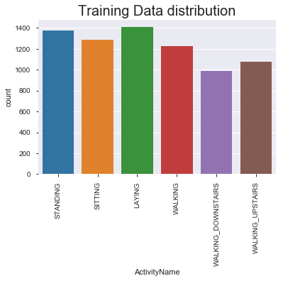
sns.countplot(train.ActivityName)
plt.title('Training Data distribution', fontsize=20)
plt.xticks(rotation=90)
plt.show()
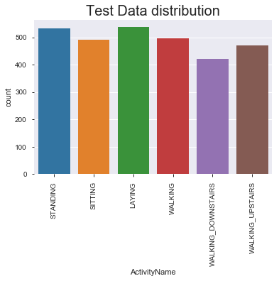
sns.countplot(test.ActivityName)
plt.title('Test Data distribution', fontsize=20)
plt.xticks(rotation=90)
plt.show()
#Observation:
# data is normally distributed in each of the activity
Duplicate data?
print ("No of duplicates in train data", sum(train.duplicated()))
print ("No of duplicates in test data", sum(test.duplicated()))
No of duplicates in train data 0
No of duplicates in test data 0
NULL data?
print ("No of null in train data", train.isnull().values.sum())
print ("No of null in test data", train.isnull().values.sum())
No of null in train data 0
No of null in test data 0
Applying t-SNE
import numpy as np
from sklearn.manifold import TSNE
import matplotlib.pyplot as plt
import seaborn as sns
def perform_tsne(X_data, y_data, perplexities, n_iter=1000, img_name_prefix='t-sne'):
for index,perplexity in enumerate(perplexities):
# perform t-sne
print('\nperforming tsne with perplexity {} and with {} iterations at max'.format(perplexity, n_iter))
X_reduced = TSNE(verbose=2, perplexity=perplexity).fit_transform(X_data)
print('Done..')
# prepare the data for seaborn
print('Creating plot for this t-sne visualization..')
df = pd.DataFrame({'x':X_reduced[:,0], 'y':X_reduced[:,1] ,'label':y_data})
# draw the plot in appropriate place in the grid
sns.lmplot(data=df, x='x', y='y', hue='label', fit_reg=False, size=8,\
palette="Set1",markers=['^','v','s','o', '1','2'])
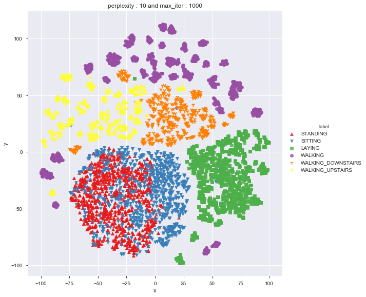
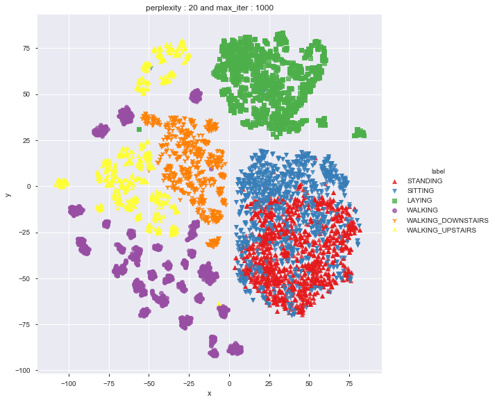
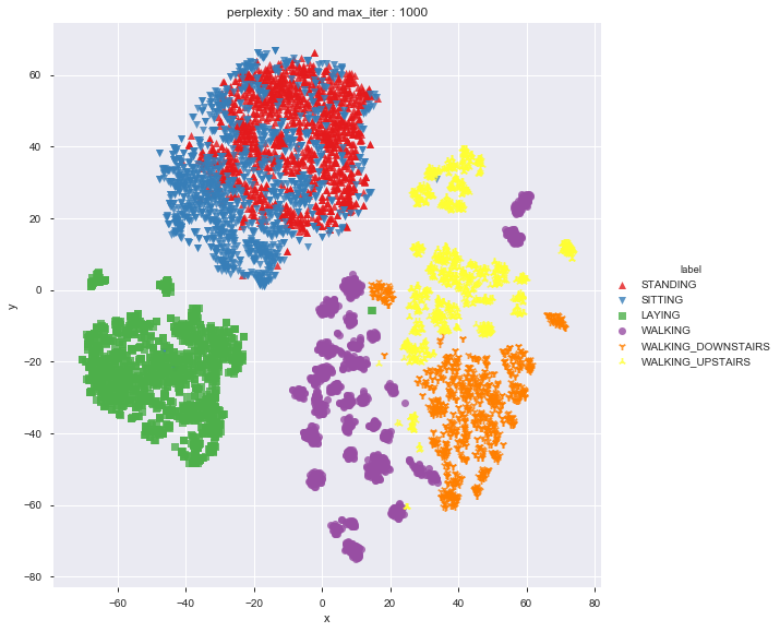
plt.title("perplexity : {} and max_iter : {}".format(perplexity, n_iter))
img_name = img_name_prefix + '_perp_{}_iter_{}.png'.format(perplexity, n_iter)
print('saving this plot as image in present working directory...')
plt.savefig(img_name)
plt.show()
print('Done')
X_pre_tsne = train.drop(['subject', 'Activity','ActivityName'], axis=1)
y_pre_tsne = train['ActivityName']
perform_tsne(X_data = X_pre_tsne,y_data=y_pre_tsne, perplexities =[2,5,10,20,50])
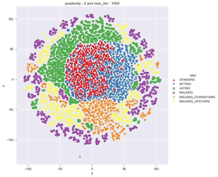
performing tsne with perplexity 2 and with 1000 iterations at max
[t-SNE] Computing 7 nearest neighbors...
[t-SNE] Indexed 7352 samples in 0.308s...
[t-SNE] Computed neighbors for 7352 samples in 41.693s...
[t-SNE] Computed conditional probabilities for sample 1000 / 7352
[t-SNE] Computed conditional probabilities for sample 2000 / 7352
[t-SNE] Computed conditional probabilities for sample 3000 / 7352
[t-SNE] Computed conditional probabilities for sample 4000 / 7352
[t-SNE] Computed conditional probabilities for sample 5000 / 7352
[t-SNE] Computed conditional probabilities for sample 6000 / 7352
[t-SNE] Computed conditional probabilities for sample 7000 / 7352
[t-SNE] Computed conditional probabilities for sample 7352 / 7352
[t-SNE] Mean sigma: 0.635855
[t-SNE] Computed conditional probabilities in 0.030s
[t-SNE] Iteration 50: error = 124.7306442, gradient norm = 0.0254025 (50 iterations in 10.484s)
[t-SNE] Iteration 100: error = 107.4000168, gradient norm = 0.0277484 (50 iterations in 3.854s)
[t-SNE] Iteration 150: error = 101.1907120, gradient norm = 0.0194172 (50 iterations in 2.700s)
[t-SNE] Iteration 200: error = 97.7570953, gradient norm = 0.0165162 (50 iterations in 2.582s)
[t-SNE] Iteration 250: error = 95.4152451, gradient norm = 0.0122675 (50 iterations in 2.545s)
[t-SNE] KL divergence after 250 iterations with early exaggeration: 95.415245
[t-SNE] Iteration 300: error = 4.1208992, gradient norm = 0.0015598 (50 iterations in 2.350s)
[t-SNE] Iteration 350: error = 3.2118182, gradient norm = 0.0010136 (50 iterations in 2.145s)
[t-SNE] Iteration 400: error = 2.7839186, gradient norm = 0.0007234 (50 iterations in 2.150s)
[t-SNE] Iteration 450: error = 2.5201564, gradient norm = 0.0005722 (50 iterations in 2.191s)
[t-SNE] Iteration 500: error = 2.3370090, gradient norm = 0.0004819 (50 iterations in 2.372s)
[t-SNE] Iteration 550: error = 2.1994641, gradient norm = 0.0004140 (50 iterations in 2.215s)
[t-SNE] Iteration 600: error = 2.0898516, gradient norm = 0.0003688 (50 iterations in 2.306s)
[t-SNE] Iteration 650: error = 1.9999684, gradient norm = 0.0003323 (50 iterations in 2.258s)
[t-SNE] Iteration 700: error = 1.9244269, gradient norm = 0.0003042 (50 iterations in 2.350s)
[t-SNE] Iteration 750: error = 1.8596187, gradient norm = 0.0002787 (50 iterations in 2.288s)
[t-SNE] Iteration 800: error = 1.8028581, gradient norm = 0.0002581 (50 iterations in 2.278s)
[t-SNE] Iteration 850: error = 1.7527609, gradient norm = 0.0002424 (50 iterations in 2.344s)
[t-SNE] Iteration 900: error = 1.7081653, gradient norm = 0.0002223 (50 iterations in 2.375s)
[t-SNE] Iteration 950: error = 1.6681588, gradient norm = 0.0002086 (50 iterations in 2.323s)
[t-SNE] Iteration 1000: error = 1.6318105, gradient norm = 0.0001985 (50 iterations in 2.329s)
[t-SNE] KL divergence after 1000 iterations: 1.631811
Done..
Creating plot for this t-sne visualization..


saving this plot as image in present working directory...
Done
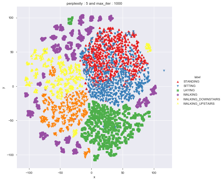
performing tsne with perplexity 5 and with 1000 iterations at max
[t-SNE] Computing 16 nearest neighbors...
[t-SNE] Indexed 7352 samples in 0.319s...
[t-SNE] Computed neighbors for 7352 samples in 40.030s...
[t-SNE] Computed conditional probabilities for sample 1000 / 7352
[t-SNE] Computed conditional probabilities for sample 2000 / 7352
[t-SNE] Computed conditional probabilities for sample 3000 / 7352
[t-SNE] Computed conditional probabilities for sample 4000 / 7352
[t-SNE] Computed conditional probabilities for sample 5000 / 7352
[t-SNE] Computed conditional probabilities for sample 6000 / 7352
[t-SNE] Computed conditional probabilities for sample 7000 / 7352
[t-SNE] Computed conditional probabilities for sample 7352 / 7352
[t-SNE] Mean sigma: 0.961265
[t-SNE] Computed conditional probabilities in 0.049s
[t-SNE] Iteration 50: error = 114.0037079, gradient norm = 0.0223941 (50 iterations in 8.132s)
[t-SNE] Iteration 100: error = 97.1023026, gradient norm = 0.0125466 (50 iterations in 3.233s)
[t-SNE] Iteration 150: error = 92.9607391, gradient norm = 0.0089509 (50 iterations in 2.391s)
[t-SNE] Iteration 200: error = 91.0669861, gradient norm = 0.0069059 (50 iterations in 2.135s)
[t-SNE] Iteration 250: error = 89.9012527, gradient norm = 0.0054905 (50 iterations in 2.104s)
[t-SNE] KL divergence after 250 iterations with early exaggeration: 89.901253
[t-SNE] Iteration 300: error = 3.5725019, gradient norm = 0.0014686 (50 iterations in 2.178s)
[t-SNE] Iteration 350: error = 2.8140268, gradient norm = 0.0007496 (50 iterations in 2.090s)
[t-SNE] Iteration 400: error = 2.4322224, gradient norm = 0.0005240 (50 iterations in 2.172s)
[t-SNE] Iteration 450: error = 2.2138059, gradient norm = 0.0004072 (50 iterations in 2.126s)
[t-SNE] Iteration 500: error = 2.0686839, gradient norm = 0.0003291 (50 iterations in 2.227s)
[t-SNE] Iteration 550: error = 1.9629487, gradient norm = 0.0002860 (50 iterations in 2.378s)
[t-SNE] Iteration 600: error = 1.8816700, gradient norm = 0.0002476 (50 iterations in 2.348s)
[t-SNE] Iteration 650: error = 1.8164161, gradient norm = 0.0002176 (50 iterations in 2.229s)
[t-SNE] Iteration 700: error = 1.7624850, gradient norm = 0.0001978 (50 iterations in 2.152s)
[t-SNE] Iteration 750: error = 1.7170402, gradient norm = 0.0001799 (50 iterations in 2.190s)
[t-SNE] Iteration 800: error = 1.6781983, gradient norm = 0.0001652 (50 iterations in 2.164s)
[t-SNE] Iteration 850: error = 1.6444139, gradient norm = 0.0001526 (50 iterations in 2.181s)
[t-SNE] Iteration 900: error = 1.6146787, gradient norm = 0.0001418 (50 iterations in 2.182s)
[t-SNE] Iteration 950: error = 1.5883613, gradient norm = 0.0001346 (50 iterations in 2.187s)
[t-SNE] Iteration 1000: error = 1.5649576, gradient norm = 0.0001259 (50 iterations in 2.172s)
[t-SNE] KL divergence after 1000 iterations: 1.564958
Done..
Creating plot for this t-sne visualization..
saving this plot as image in present working directory...
Done

performing tsne with perplexity 10 and with 1000 iterations at max
[t-SNE] Computing 31 nearest neighbors...
[t-SNE] Indexed 7352 samples in 0.286s...
[t-SNE] Computed neighbors for 7352 samples in 40.628s...
[t-SNE] Computed conditional probabilities for sample 1000 / 7352
[t-SNE] Computed conditional probabilities for sample 2000 / 7352
[t-SNE] Computed conditional probabilities for sample 3000 / 7352
[t-SNE] Computed conditional probabilities for sample 4000 / 7352
[t-SNE] Computed conditional probabilities for sample 5000 / 7352
[t-SNE] Computed conditional probabilities for sample 6000 / 7352
[t-SNE] Computed conditional probabilities for sample 7000 / 7352
[t-SNE] Computed conditional probabilities for sample 7352 / 7352
[t-SNE] Mean sigma: 1.133828
[t-SNE] Computed conditional probabilities in 0.093s
[t-SNE] Iteration 50: error = 105.4349060, gradient norm = 0.0228049 (50 iterations in 3.940s)
[t-SNE] Iteration 100: error = 90.0550919, gradient norm = 0.0104028 (50 iterations in 2.665s)
[t-SNE] Iteration 150: error = 87.1365509, gradient norm = 0.0061813 (50 iterations in 2.446s)
[t-SNE] Iteration 200: error = 85.9506378, gradient norm = 0.0037276 (50 iterations in 2.506s)
[t-SNE] Iteration 250: error = 85.2917557, gradient norm = 0.0030748 (50 iterations in 2.501s)
[t-SNE] KL divergence after 250 iterations with early exaggeration: 85.291756
[t-SNE] Iteration 300: error = 3.1292915, gradient norm = 0.0013841 (50 iterations in 2.282s)
[t-SNE] Iteration 350: error = 2.4879830, gradient norm = 0.0006477 (50 iterations in 2.140s)
[t-SNE] Iteration 400: error = 2.1684470, gradient norm = 0.0004229 (50 iterations in 2.168s)
[t-SNE] Iteration 450: error = 1.9844533, gradient norm = 0.0003159 (50 iterations in 2.213s)
[t-SNE] Iteration 500: error = 1.8669348, gradient norm = 0.0002521 (50 iterations in 2.228s)
[t-SNE] Iteration 550: error = 1.7840797, gradient norm = 0.0002120 (50 iterations in 2.300s)
[t-SNE] Iteration 600: error = 1.7218199, gradient norm = 0.0001813 (50 iterations in 2.262s)
[t-SNE] Iteration 650: error = 1.6728977, gradient norm = 0.0001612 (50 iterations in 2.356s)
[t-SNE] Iteration 700: error = 1.6335385, gradient norm = 0.0001425 (50 iterations in 2.216s)
[t-SNE] Iteration 750: error = 1.6009146, gradient norm = 0.0001291 (50 iterations in 2.340s)
[t-SNE] Iteration 800: error = 1.5735505, gradient norm = 0.0001195 (50 iterations in 2.293s)
[t-SNE] Iteration 850: error = 1.5499940, gradient norm = 0.0001114 (50 iterations in 2.275s)
[t-SNE] Iteration 900: error = 1.5297399, gradient norm = 0.0001043 (50 iterations in 2.343s)
[t-SNE] Iteration 950: error = 1.5122747, gradient norm = 0.0000970 (50 iterations in 2.270s)
[t-SNE] Iteration 1000: error = 1.4971433, gradient norm = 0.0000928 (50 iterations in 2.327s)
[t-SNE] KL divergence after 1000 iterations: 1.497143
Done..
Creating plot for this t-sne visualization..


saving this plot as image in present working directory...
Done

performing tsne with perplexity 20 and with 1000 iterations at max
[t-SNE] Computing 61 nearest neighbors...
[t-SNE] Indexed 7352 samples in 0.297s...
[t-SNE] Computed neighbors for 7352 samples in 40.723s...
[t-SNE] Computed conditional probabilities for sample 1000 / 7352
[t-SNE] Computed conditional probabilities for sample 2000 / 7352
[t-SNE] Computed conditional probabilities for sample 3000 / 7352
[t-SNE] Computed conditional probabilities for sample 4000 / 7352
[t-SNE] Computed conditional probabilities for sample 5000 / 7352
[t-SNE] Computed conditional probabilities for sample 6000 / 7352
[t-SNE] Computed conditional probabilities for sample 7000 / 7352
[t-SNE] Computed conditional probabilities for sample 7352 / 7352
[t-SNE] Mean sigma: 1.274335
[t-SNE] Computed conditional probabilities in 0.187s
[t-SNE] Iteration 50: error = 96.6237259, gradient norm = 0.0274812 (50 iterations in 4.596s)
[t-SNE] Iteration 100: error = 83.9835892, gradient norm = 0.0058667 (50 iterations in 3.090s)
[t-SNE] Iteration 150: error = 81.9641571, gradient norm = 0.0037054 (50 iterations in 12.441s)
[t-SNE] Iteration 200: error = 81.2029266, gradient norm = 0.0027636 (50 iterations in 7.540s)
[t-SNE] Iteration 250: error = 80.8060989, gradient norm = 0.0023002 (50 iterations in 6.325s)
[t-SNE] KL divergence after 250 iterations with early exaggeration: 80.806099
[t-SNE] Iteration 300: error = 2.6924877, gradient norm = 0.0012978 (50 iterations in 4.996s)
[t-SNE] Iteration 350: error = 2.1620288, gradient norm = 0.0005745 (50 iterations in 3.987s)
[t-SNE] Iteration 400: error = 1.9130983, gradient norm = 0.0003475 (50 iterations in 3.610s)
[t-SNE] Iteration 450: error = 1.7667772, gradient norm = 0.0002478 (50 iterations in 3.787s)
[t-SNE] Iteration 500: error = 1.6730547, gradient norm = 0.0001905 (50 iterations in 3.154s)
[t-SNE] Iteration 550: error = 1.6090366, gradient norm = 0.0001575 (50 iterations in 2.709s)
[t-SNE] Iteration 600: error = 1.5625103, gradient norm = 0.0001329 (50 iterations in 2.400s)
[t-SNE] Iteration 650: error = 1.5270337, gradient norm = 0.0001159 (50 iterations in 2.470s)
[t-SNE] Iteration 700: error = 1.4995929, gradient norm = 0.0001044 (50 iterations in 2.398s)
[t-SNE] Iteration 750: error = 1.4777728, gradient norm = 0.0000953 (50 iterations in 2.526s)
[t-SNE] Iteration 800: error = 1.4598433, gradient norm = 0.0000897 (50 iterations in 2.524s)
[t-SNE] Iteration 850: error = 1.4454199, gradient norm = 0.0000831 (50 iterations in 2.426s)
[t-SNE] Iteration 900: error = 1.4334183, gradient norm = 0.0000806 (50 iterations in 2.431s)
[t-SNE] Iteration 950: error = 1.4237714, gradient norm = 0.0000755 (50 iterations in 2.410s)
[t-SNE] Iteration 1000: error = 1.4159596, gradient norm = 0.0000740 (50 iterations in 2.453s)
[t-SNE] KL divergence after 1000 iterations: 1.415960
Done..
Creating plot for this t-sne visualization..


saving this plot as image in present working directory...
Done

performing tsne with perplexity 50 and with 1000 iterations at max
[t-SNE] Computing 151 nearest neighbors...
[t-SNE] Indexed 7352 samples in 0.273s...
[t-SNE] Computed neighbors for 7352 samples in 40.643s...
[t-SNE] Computed conditional probabilities for sample 1000 / 7352
[t-SNE] Computed conditional probabilities for sample 2000 / 7352
[t-SNE] Computed conditional probabilities for sample 3000 / 7352
[t-SNE] Computed conditional probabilities for sample 4000 / 7352
[t-SNE] Computed conditional probabilities for sample 5000 / 7352
[t-SNE] Computed conditional probabilities for sample 6000 / 7352
[t-SNE] Computed conditional probabilities for sample 7000 / 7352
[t-SNE] Computed conditional probabilities for sample 7352 / 7352
[t-SNE] Mean sigma: 1.437672
[t-SNE] Computed conditional probabilities in 0.416s
[t-SNE] Iteration 50: error = 86.4786377, gradient norm = 0.0187448 (50 iterations in 5.873s)
[t-SNE] Iteration 100: error = 75.6487274, gradient norm = 0.0046881 (50 iterations in 4.415s)
[t-SNE] Iteration 150: error = 74.6104736, gradient norm = 0.0021831 (50 iterations in 3.506s)
[t-SNE] Iteration 200: error = 74.2436523, gradient norm = 0.0015965 (50 iterations in 3.881s)
[t-SNE] Iteration 250: error = 74.0575638, gradient norm = 0.0011124 (50 iterations in 3.527s)
[t-SNE] KL divergence after 250 iterations with early exaggeration: 74.057564
[t-SNE] Iteration 300: error = 2.1557598, gradient norm = 0.0011830 (50 iterations in 3.679s)
[t-SNE] Iteration 350: error = 1.7585902, gradient norm = 0.0004913 (50 iterations in 3.118s)
[t-SNE] Iteration 400: error = 1.5895849, gradient norm = 0.0002805 (50 iterations in 3.481s)
[t-SNE] Iteration 450: error = 1.4958792, gradient norm = 0.0001877 (50 iterations in 3.254s)
[t-SNE] Iteration 500: error = 1.4360178, gradient norm = 0.0001417 (50 iterations in 3.216s)
[t-SNE] Iteration 550: error = 1.3948883, gradient norm = 0.0001115 (50 iterations in 3.418s)
[t-SNE] Iteration 600: error = 1.3656672, gradient norm = 0.0000940 (50 iterations in 3.619s)
[t-SNE] Iteration 650: error = 1.3443383, gradient norm = 0.0000845 (50 iterations in 3.451s)
[t-SNE] Iteration 700: error = 1.3286852, gradient norm = 0.0000757 (50 iterations in 3.473s)
[t-SNE] Iteration 750: error = 1.3170402, gradient norm = 0.0000696 (50 iterations in 3.312s)
[t-SNE] Iteration 800: error = 1.3080970, gradient norm = 0.0000720 (50 iterations in 3.315s)
[t-SNE] Iteration 850: error = 1.3014609, gradient norm = 0.0000626 (50 iterations in 3.458s)
[t-SNE] Iteration 900: error = 1.2959986, gradient norm = 0.0000589 (50 iterations in 3.321s)
[t-SNE] Iteration 950: error = 1.2915746, gradient norm = 0.0000551 (50 iterations in 3.526s)
[t-SNE] Iteration 1000: error = 1.2878189, gradient norm = 0.0000535 (50 iterations in 3.158s)
[t-SNE] KL divergence after 1000 iterations: 1.287819
Done..
Creating plot for this t-sne visualization..


saving this plot as image in present working directory...
Done
As per t-sne, it seems to be difficult to differentiate between standing and sitting
Modelling
train.head()
| tBodyAccmeanX | tBodyAccmeanY | tBodyAccmeanZ | tBodyAccstdX | tBodyAccstdY | tBodyAccstdZ | tBodyAccmadX | tBodyAccmadY | tBodyAccmadZ | tBodyAccmaxX | ... | angletBodyAccMeangravity | angletBodyAccJerkMeangravityMean | angletBodyGyroMeangravityMean | angletBodyGyroJerkMeangravityMean | angleXgravityMean | angleYgravityMean | angleZgravityMean | subject | Activity | ActivityName | |
|---|---|---|---|---|---|---|---|---|---|---|---|---|---|---|---|---|---|---|---|---|---|
| 0 | 0.288585 | -0.020294 | -0.132905 | -0.995279 | -0.983111 | -0.913526 | -0.995112 | -0.983185 | -0.923527 | -0.934724 | ... | -0.112754 | 0.030400 | -0.464761 | -0.018446 | -0.841247 | 0.179941 | -0.058627 | 1 | 5 | STANDING |
| 1 | 0.278419 | -0.016411 | -0.123520 | -0.998245 | -0.975300 | -0.960322 | -0.998807 | -0.974914 | -0.957686 | -0.943068 | ... | 0.053477 | -0.007435 | -0.732626 | 0.703511 | -0.844788 | 0.180289 | -0.054317 | 1 | 5 | STANDING |
| 2 | 0.279653 | -0.019467 | -0.113462 | -0.995380 | -0.967187 | -0.978944 | -0.996520 | -0.963668 | -0.977469 | -0.938692 | ... | -0.118559 | 0.177899 | 0.100699 | 0.808529 | -0.848933 | 0.180637 | -0.049118 | 1 | 5 | STANDING |
| 3 | 0.279174 | -0.026201 | -0.123283 | -0.996091 | -0.983403 | -0.990675 | -0.997099 | -0.982750 | -0.989302 | -0.938692 | ... | -0.036788 | -0.012892 | 0.640011 | -0.485366 | -0.848649 | 0.181935 | -0.047663 | 1 | 5 | STANDING |
| 4 | 0.276629 | -0.016570 | -0.115362 | -0.998139 | -0.980817 | -0.990482 | -0.998321 | -0.979672 | -0.990441 | -0.942469 | ... | 0.123320 | 0.122542 | 0.693578 | -0.615971 | -0.847865 | 0.185151 | -0.043892 | 1 | 5 | STANDING |
5 rows × 564 columns
X_train = train.drop(['subject', 'Activity', 'ActivityName'], axis=1)
y_train = train.ActivityName
X_test = test.drop(['subject', 'Activity', 'ActivityName'], axis=1)
y_test = test.ActivityName
labels=['LAYING', 'SITTING','STANDING','WALKING','WALKING_DOWNSTAIRS','WALKING_UPSTAIRS']
from sklearn.linear_model import LogisticRegression
model = LogisticRegression(C=10)
model
LogisticRegression(C=10, class_weight=None, dual=False, fit_intercept=True,
          intercept_scaling=1, max_iter=100, multi_class='warn',
          n_jobs=None, penalty='l2', random_state=None, solver='warn',
          tol=0.0001, verbose=0, warm_start=False)
model.fit(X_train, y_train)
LogisticRegression(C=10, class_weight=None, dual=False, fit_intercept=True,
          intercept_scaling=1, max_iter=100, multi_class='warn',
          n_jobs=None, penalty='l2', random_state=None, solver='warn',
          tol=0.0001, verbose=0, warm_start=False)
model.score(X_test, y_test)
0.9619952494061758
from sklearn.model_selection import GridSearchCV
parameters = {'C':[0.01, 0.1, 1, 10, 20, 30], 'penalty':['l2','l1']}
model_cv = GridSearchCV(model, param_grid=parameters, cv=3, verbose=1, n_jobs=-1)
model_cv.fit(X_train, y_train)
Fitting 3 folds for each of 12 candidates, totalling 36 fits


[Parallel(n_jobs=-1)]: Using backend LokyBackend with 8 concurrent workers.
[Parallel(n_jobs=-1)]: Done  36 out of  36 | elapsed:   49.6s finished


GridSearchCV(cv=3, error_score='raise-deprecating',
       estimator=LogisticRegression(C=10, class_weight=None, dual=False, fit_intercept=True,
          intercept_scaling=1, max_iter=100, multi_class='warn',
          n_jobs=None, penalty='l2', random_state=None, solver='warn',
          tol=0.0001, verbose=0, warm_start=False),
       fit_params=None, iid='warn', n_jobs=-1,
       param_grid={'C': [0.01, 0.1, 1, 10, 20, 30], 'penalty': ['l2', 'l1']},
       pre_dispatch='2*n_jobs', refit=True, return_train_score='warn',
       scoring=None, verbose=1)
from sklearn.metrics import classification_report
print (classification_report(model_cv.best_estimator_.predict(X_test), y_test))
                    precision    recall  f1-score   support

            LAYING       1.00      1.00      1.00       538
           SITTING       0.87      0.97      0.92       440
          STANDING       0.98      0.90      0.94       577
           WALKING       1.00      0.95      0.97       521
WALKING_DOWNSTAIRS       0.97      1.00      0.99       410
  WALKING_UPSTAIRS       0.95      0.97      0.96       461

         micro avg       0.96      0.96      0.96      2947
         macro avg       0.96      0.97      0.96      2947
      weighted avg       0.96      0.96      0.96      2947
from sklearn.metrics import confusion_matrix
import itertools
import numpy as np
import matplotlib.pyplot as plt
from sklearn.metrics import confusion_matrix
plt.rcParams["font.family"] = 'DejaVu Sans'

def plot_confusion_matrix(cm, classes,
                          normalize=False,
                          title='Confusion matrix',
                          cmap=plt.cm.Blues):
    if normalize:
        cm = cm.astype('float') / cm.sum(axis=1)[:, np.newaxis]

    plt.imshow(cm, interpolation='nearest', cmap=cmap)
    plt.title(title)
    plt.colorbar()
    tick_marks = np.arange(len(classes))
    plt.xticks(tick_marks, classes, rotation=90)
    plt.yticks(tick_marks, classes)

    fmt = '.2f' if normalize else 'd'
    thresh = cm.max() / 2.
    for i, j in itertools.product(range(cm.shape[0]), range(cm.shape[1])):
        plt.text(j, i, format(cm[i, j], fmt),
                 horizontalalignment="center",
                 color="white" if cm[i, j] > thresh else "black")

    plt.tight_layout()
    plt.ylabel('True label')
    plt.xlabel('Predicted label')
from datetime import datetime
def perform_model(model, X_train, y_train, X_test, y_test, class_labels, cm_normalize=True, \
                 print_cm=True, cm_cmap=plt.cm.Greens):


    # to store results at various phases
    results = dict()

    # time at which model starts training
    train_start_time = datetime.now()
    print('training the model..')
    model.fit(X_train, y_train)
    print('Done \n \n')
    train_end_time = datetime.now()
    results['training_time'] =  train_end_time - train_start_time
    print('training_time(HH:MM:SS.ms) - {}\n\n'.format(results['training_time']))


    # predict test data
    print('Predicting test data')
    test_start_time = datetime.now()
    y_pred = model.predict(X_test)
    test_end_time = datetime.now()
    print('Done \n \n')
    results['testing_time'] = test_end_time - test_start_time
    print('testing time(HH:MM:SS:ms) - {}\n\n'.format(results['testing_time']))
    results['predicted'] = y_pred


    # calculate overall accuracty of the model
    accuracy = metrics.accuracy_score(y_true=y_test, y_pred=y_pred)
    # store accuracy in results
    results['accuracy'] = accuracy
    print('---------------------')
    print('|      Accuracy      |')
    print('---------------------')
    print('\n    {}\n\n'.format(accuracy))


    # confusion matrix
    cm = metrics.confusion_matrix(y_test, y_pred)
    results['confusion_matrix'] = cm
    if print_cm:
        print('--------------------')
        print('| Confusion Matrix |')
        print('--------------------')
        print('\n {}'.format(cm))

    # plot confusin matrix
    plt.figure(figsize=(8,8))
    plt.grid(b=False)
    plot_confusion_matrix(cm, classes=class_labels, normalize=True, title='Normalized confusion matrix', cmap = cm_cmap)
    plt.show()

    # get classification report
    print('-------------------------')
    print('| Classifiction Report |')
    print('-------------------------')
    classification_report = metrics.classification_report(y_test, y_pred)
    # store report in results
    results['classification_report'] = classification_report
    print(classification_report)

    # add the trained  model to the results
    results['model'] = model

    return results
def print_grid_search_attributes(model):
    # Estimator that gave highest score among all the estimators formed in GridSearch
    print('--------------------------')
    print('|      Best Estimator     |')
    print('--------------------------')
    print('\n\t{}\n'.format(model.best_estimator_))


    # parameters that gave best results while performing grid search
    print('--------------------------')
    print('|     Best parameters     |')
    print('--------------------------')
    print('\tParameters of best estimator : \n\n\t{}\n'.format(model.best_params_))


    #  number of cross validation splits
    print('---------------------------------')
    print('|   No of CrossValidation sets   |')
    print('--------------------------------')
    print('\n\tTotal numbre of cross validation sets: {}\n'.format(model.n_splits_))


    # Average cross validated score of the best estimator, from the Grid Search
    print('--------------------------')
    print('|        Best Score       |')
    print('--------------------------')
    print('\n\tAverage Cross Validate scores of best estimator : \n\n\t{}\n'.format(model.best_score_))
Logistic Regression with Grid Search
from sklearn import linear_model
from sklearn import metrics

from sklearn.model_selection import GridSearchCV
# start Grid search
import warnings
warnings.filterwarnings('ignore')

parameters = {'C':[0.01, 0.1, 1, 10, 20, 30], 'penalty':['l2','l1']}
log_reg = linear_model.LogisticRegression()
log_reg_grid = GridSearchCV(log_reg, param_grid=parameters, cv=3, verbose=1, n_jobs=-1)
log_reg_grid_results =  perform_model(log_reg_grid, X_train, y_train, X_test, y_test, class_labels=labels)
training the model..
Fitting 3 folds for each of 12 candidates, totalling 36 fits


[Parallel(n_jobs=-1)]: Using backend LokyBackend with 8 concurrent workers.
[Parallel(n_jobs=-1)]: Done  36 out of  36 | elapsed:   53.0s finished


Done


training_time(HH:MM:SS.ms) - 0:01:00.286430


Predicting test data
Done


testing time(HH:MM:SS:ms) - 0:00:00.005971


---------------------
|      Accuracy      |
---------------------

    0.9626739056667798


--------------------
| Confusion Matrix |
--------------------

 [[537   0   0   0   0   0]
 [  1 428  58   0   0   4]
 [  0  12 519   1   0   0]
 [  0   0   0 495   1   0]
 [  0   0   0   3 409   8]
 [  0   0   0  22   0 449]]

-------------------------
| Classifiction Report |
-------------------------
                    precision    recall  f1-score   support

            LAYING       1.00      1.00      1.00       537
           SITTING       0.97      0.87      0.92       491
          STANDING       0.90      0.98      0.94       532
           WALKING       0.95      1.00      0.97       496
WALKING_DOWNSTAIRS       1.00      0.97      0.99       420
  WALKING_UPSTAIRS       0.97      0.95      0.96       471

         micro avg       0.96      0.96      0.96      2947
         macro avg       0.97      0.96      0.96      2947
      weighted avg       0.96      0.96      0.96      2947
# observe the attributes of the model
print_grid_search_attributes(log_reg_grid_results['model'])
--------------------------
|      Best Estimator     |
--------------------------

	LogisticRegression(C=30, class_weight=None, dual=False, fit_intercept=True,
          intercept_scaling=1, max_iter=100, multi_class='warn',
          n_jobs=None, penalty='l2', random_state=None, solver='warn',
          tol=0.0001, verbose=0, warm_start=False)

--------------------------
|     Best parameters     |
--------------------------
	Parameters of best estimator :

	{'C': 30, 'penalty': 'l2'}

---------------------------------
|   No of CrossValidation sets   |
--------------------------------

	Total numbre of cross validation sets: 3

--------------------------
|        Best Score       |
--------------------------

	Average Cross Validate scores of best estimator :

	0.9461371055495104
Linear SVC
from sklearn.svm import LinearSVC
parameters = {'C':[0.125, 0.5, 1, 2, 8, 16]}
lr_svc = LinearSVC()
lr_svc_grid = GridSearchCV(lr_svc, param_grid=parameters, n_jobs=-1, verbose=1)
lr_svc_grid_results = perform_model(lr_svc_grid, X_train, y_train, X_test, y_test, class_labels=labels)
training the model..
Fitting 3 folds for each of 6 candidates, totalling 18 fits


[Parallel(n_jobs=-1)]: Using backend LokyBackend with 8 concurrent workers.
[Parallel(n_jobs=-1)]: Done  18 out of  18 | elapsed:   16.3s finished


Done


training_time(HH:MM:SS.ms) - 0:00:20.944422


Predicting test data
Done


testing time(HH:MM:SS:ms) - 0:00:00.005967


---------------------
|      Accuracy      |
---------------------

    0.9569053274516457


--------------------
| Confusion Matrix |
--------------------

 [[537   0   0   0   0   0]
 [  1 392  93   0   0   5]
 [  0   3 528   1   0   0]
 [  0   0   0 496   0   0]
 [  0   0   0   2 413   5]
 [  0   0   0  16   1 454]]
-------------------------
| Classifiction Report |
-------------------------
                    precision    recall  f1-score   support

            LAYING       1.00      1.00      1.00       537
           SITTING       0.99      0.80      0.88       491
          STANDING       0.85      0.99      0.92       532
           WALKING       0.96      1.00      0.98       496
WALKING_DOWNSTAIRS       1.00      0.98      0.99       420
  WALKING_UPSTAIRS       0.98      0.96      0.97       471

         micro avg       0.96      0.96      0.96      2947
         macro avg       0.96      0.96      0.96      2947
      weighted avg       0.96      0.96      0.96      2947
print_grid_search_attributes(lr_svc_grid_results['model'])
--------------------------
|      Best Estimator     |
--------------------------

	LinearSVC(C=2, class_weight=None, dual=True, fit_intercept=True,
     intercept_scaling=1, loss='squared_hinge', max_iter=1000,
     multi_class='ovr', penalty='l2', random_state=None, tol=0.0001,
     verbose=0)

--------------------------
|     Best parameters     |
--------------------------
	Parameters of best estimator :

	{'C': 2}

---------------------------------
|   No of CrossValidation sets   |
--------------------------------

	Total numbre of cross validation sets: 3

--------------------------
|        Best Score       |
--------------------------

	Average Cross Validate scores of best estimator :

	0.9465451577801959
Kernal SVM with GridSearch
from sklearn.svm import SVC
parameters = {'C':[2,8,16],\
              'gamma': [ 0.0078125, 0.125, 2]}
rbf_svm = SVC(kernel='rbf')
rbf_svm_grid = GridSearchCV(rbf_svm,param_grid=parameters, n_jobs=-1)
rbf_svm_grid_results = perform_model(rbf_svm_grid, X_train, y_train, X_test, y_test, class_labels=labels)
training the model..
Done


training_time(HH:MM:SS.ms) - 0:03:51.587765


Predicting test data
Done


testing time(HH:MM:SS:ms) - 0:00:02.498984


---------------------
|      Accuracy      |
---------------------

    0.9626739056667798


--------------------
| Confusion Matrix |
--------------------

 [[537   0   0   0   0   0]
 [  0 441  48   0   0   2]
 [  0  12 520   0   0   0]
 [  0   0   0 489   2   5]
 [  0   0   0   4 397  19]
 [  0   0   0  17   1 453]]

-------------------------
| Classifiction Report |
-------------------------
                    precision    recall  f1-score   support

            LAYING       1.00      1.00      1.00       537
           SITTING       0.97      0.90      0.93       491
          STANDING       0.92      0.98      0.95       532
           WALKING       0.96      0.99      0.97       496
WALKING_DOWNSTAIRS       0.99      0.95      0.97       420
  WALKING_UPSTAIRS       0.95      0.96      0.95       471

         micro avg       0.96      0.96      0.96      2947
         macro avg       0.96      0.96      0.96      2947
      weighted avg       0.96      0.96      0.96      2947
print_grid_search_attributes(rbf_svm_grid_results['model'])
--------------------------
|      Best Estimator     |
--------------------------

	SVC(C=16, cache_size=200, class_weight=None, coef0=0.0,
  decision_function_shape='ovr', degree=3, gamma=0.0078125, kernel='rbf',
  max_iter=-1, probability=False, random_state=None, shrinking=True,
  tol=0.001, verbose=False)

--------------------------
|     Best parameters     |
--------------------------
	Parameters of best estimator :

	{'C': 16, 'gamma': 0.0078125}

---------------------------------
|   No of CrossValidation sets   |
--------------------------------

	Total numbre of cross validation sets: 3

--------------------------
|        Best Score       |
--------------------------

	Average Cross Validate scores of best estimator :

	0.9440968443960827
Decision Tree with Grid Search
from sklearn.tree import DecisionTreeClassifier
parameters = {'max_depth':np.arange(3,10,2)}
dt = DecisionTreeClassifier()
dt_grid = GridSearchCV(dt,param_grid=parameters, n_jobs=-1)
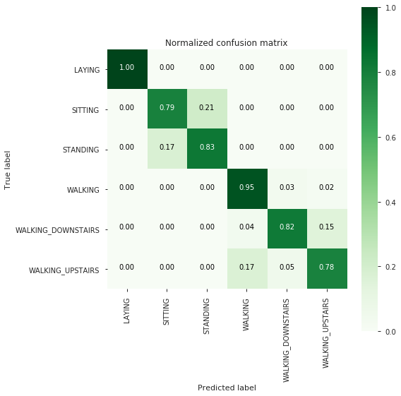
dt_grid_results = perform_model(dt_grid, X_train, y_train, X_test, y_test, class_labels=labels)
print_grid_search_attributes(dt_grid_results['model'])
training the model..
Done


training_time(HH:MM:SS.ms) - 0:00:09.535803


Predicting test data
Done


testing time(HH:MM:SS:ms) - 0:00:00.007000


---------------------
|      Accuracy      |
---------------------

    0.8642687478791992


--------------------
| Confusion Matrix |
--------------------

 [[537   0   0   0   0   0]
 [  0 386 105   0   0   0]
 [  0  93 439   0   0   0]
 [  0   0   0 472  16   8]
 [  0   0   0  15 344  61]
 [  0   0   0  78  24 369]]
-------------------------
| Classifiction Report |
-------------------------
                    precision    recall  f1-score   support

            LAYING       1.00      1.00      1.00       537
           SITTING       0.81      0.79      0.80       491
          STANDING       0.81      0.83      0.82       532
           WALKING       0.84      0.95      0.89       496
WALKING_DOWNSTAIRS       0.90      0.82      0.86       420
  WALKING_UPSTAIRS       0.84      0.78      0.81       471

         micro avg       0.86      0.86      0.86      2947
         macro avg       0.86      0.86      0.86      2947
      weighted avg       0.87      0.86      0.86      2947

--------------------------
|      Best Estimator     |
--------------------------

	DecisionTreeClassifier(class_weight=None, criterion='gini', max_depth=7,
            max_features=None, max_leaf_nodes=None,
            min_impurity_decrease=0.0, min_impurity_split=None,
            min_samples_leaf=1, min_samples_split=2,
            min_weight_fraction_leaf=0.0, presort=False, random_state=None,
            splitter='best')

--------------------------
|     Best parameters     |
--------------------------
	Parameters of best estimator :

	{'max_depth': 7}

---------------------------------
|   No of CrossValidation sets   |
--------------------------------

	Total numbre of cross validation sets: 3

--------------------------
|        Best Score       |
--------------------------

	Average Cross Validate scores of best estimator :

	0.8430359085963003
Random Forest with Grid Search
from sklearn.ensemble import RandomForestClassifier
params = {'n_estimators': np.arange(10,201,20), 'max_depth':np.arange(3,15,2)}
rfc = RandomForestClassifier()
rfc_grid = GridSearchCV(rfc, param_grid=params, n_jobs=-1)
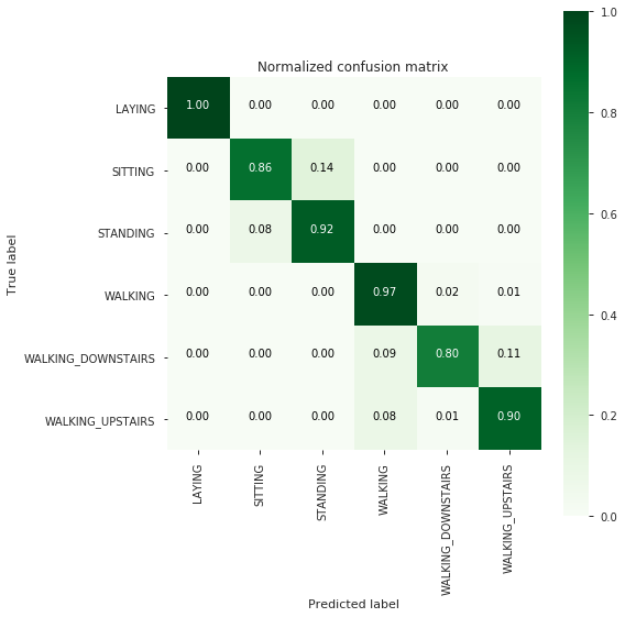
rfc_grid_results = perform_model(rfc_grid, X_train, y_train, X_test, y_test, class_labels=labels)
print_grid_search_attributes(rfc_grid_results['model'])
training the model..
Done


training_time(HH:MM:SS.ms) - 0:02:50.105956


Predicting test data
Done


testing time(HH:MM:SS:ms) - 0:00:00.035000


---------------------
|      Accuracy      |
---------------------

    0.9148286392941974


--------------------
| Confusion Matrix |
--------------------

 [[537   0   0   0   0   0]
 [  0 421  70   0   0   0]
 [  0  41 491   0   0   0]
 [  0   0   0 483  10   3]
 [  0   0   0  36 338  46]
 [  0   0   0  39   6 426]]
-------------------------
| Classifiction Report |
-------------------------
                    precision    recall  f1-score   support

            LAYING       1.00      1.00      1.00       537
           SITTING       0.91      0.86      0.88       491
          STANDING       0.88      0.92      0.90       532
           WALKING       0.87      0.97      0.92       496
WALKING_DOWNSTAIRS       0.95      0.80      0.87       420
  WALKING_UPSTAIRS       0.90      0.90      0.90       471

         micro avg       0.91      0.91      0.91      2947
         macro avg       0.92      0.91      0.91      2947
      weighted avg       0.92      0.91      0.91      2947

--------------------------
|      Best Estimator     |
--------------------------

	RandomForestClassifier(bootstrap=True, class_weight=None, criterion='gini',
            max_depth=7, max_features='auto', max_leaf_nodes=None,
            min_impurity_decrease=0.0, min_impurity_split=None,
            min_samples_leaf=1, min_samples_split=2,
            min_weight_fraction_leaf=0.0, n_estimators=90, n_jobs=None,
            oob_score=False, random_state=None, verbose=0,
            warm_start=False)

--------------------------
|     Best parameters     |
--------------------------
	Parameters of best estimator :

	{'max_depth': 7, 'n_estimators': 90}

---------------------------------
|   No of CrossValidation sets   |
--------------------------------

	Total numbre of cross validation sets: 3

--------------------------
|        Best Score       |
--------------------------

	Average Cross Validate scores of best estimator :

	0.9166213275299239
Gradient Boosting with Grid Search
from sklearn.ensemble import GradientBoostingClassifier
param_grid = {'max_depth': np.arange(5,8,1), \
'n_estimators':np.arange(130,170,10)}
gbdt = GradientBoostingClassifier()
gbdt_grid = GridSearchCV(gbdt, param_grid=param_grid, n_jobs=-1)
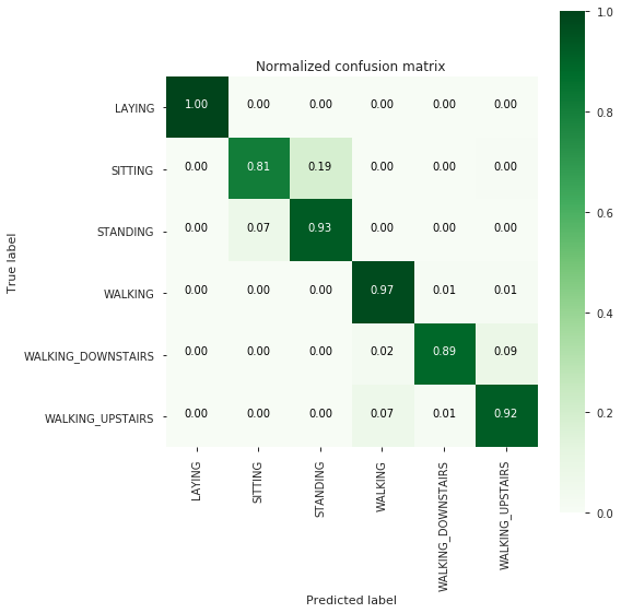
gbdt_grid_results = perform_model(gbdt_grid, X_train, y_train, X_test, y_test, class_labels=labels)
print_grid_search_attributes(gbdt_grid_results['model'])
training the model..
Done


training_time(HH:MM:SS.ms) - 0:26:26.698912


Predicting test data
Done


testing time(HH:MM:SS:ms) - 0:00:00.074994


---------------------
|      Accuracy      |
---------------------

    0.9222938581608415


--------------------
| Confusion Matrix |
--------------------

 [[537   0   0   0   0   0]
 [  0 397  92   0   0   2]
 [  0  38 494   0   0   0]
 [  0   0   0 483   7   6]
 [  0   0   0  10 374  36]
 [  0   1   0  31   6 433]]
-------------------------
| Classifiction Report |
-------------------------
                    precision    recall  f1-score   support

            LAYING       1.00      1.00      1.00       537
           SITTING       0.91      0.81      0.86       491
          STANDING       0.84      0.93      0.88       532
           WALKING       0.92      0.97      0.95       496
WALKING_DOWNSTAIRS       0.97      0.89      0.93       420
  WALKING_UPSTAIRS       0.91      0.92      0.91       471

         micro avg       0.92      0.92      0.92      2947
         macro avg       0.92      0.92      0.92      2947
      weighted avg       0.92      0.92      0.92      2947

--------------------------
|      Best Estimator     |
--------------------------

	GradientBoostingClassifier(criterion='friedman_mse', init=None,
              learning_rate=0.1, loss='deviance', max_depth=5,
              max_features=None, max_leaf_nodes=None,
              min_impurity_decrease=0.0, min_impurity_split=None,
              min_samples_leaf=1, min_samples_split=2,
              min_weight_fraction_leaf=0.0, n_estimators=160,
              n_iter_no_change=None, presort='auto', random_state=None,
              subsample=1.0, tol=0.0001, validation_fraction=0.1,
              verbose=0, warm_start=False)

--------------------------
|     Best parameters     |
--------------------------
	Parameters of best estimator :

	{'max_depth': 5, 'n_estimators': 160}

---------------------------------
|   No of CrossValidation sets   |
--------------------------------

	Total numbre of cross validation sets: 3

--------------------------
|        Best Score       |
--------------------------

	Average Cross Validate scores of best estimator :

	0.904923830250272
KNN with GridSearch
from sklearn.neighbors import KNeighborsClassifier
param_grid = {'n_neighbors': [5, 10, 15, 20, 25]}
knn = KNeighborsClassifier()
knn_grid = GridSearchCV(knn, param_grid=param_grid, n_jobs=-1)
knn_grid_results = perform_model(knn_grid, X_train, y_train, X_test, y_test, class_labels=labels)
print_grid_search_attributes(knn_grid_results['model'])
training the model..
Done


training_time(HH:MM:SS.ms) - 0:01:48.987910


Predicting test data
Done


testing time(HH:MM:SS:ms) - 0:00:15.102018


---------------------
|      Accuracy      |
---------------------

    0.9056667797760435


--------------------
| Confusion Matrix |
--------------------

 [[535   1   1   0   0   0]
 [  0 400  87   0   0   4]
 [  0  37 495   0   0   0]
 [  0   0   0 489   7   0]
 [  0   0   0  53 325  42]
 [  0   0   0  41   5 425]]
-------------------------
| Classifiction Report |
-------------------------
                    precision    recall  f1-score   support

            LAYING       1.00      1.00      1.00       537
           SITTING       0.91      0.81      0.86       491
          STANDING       0.85      0.93      0.89       532
           WALKING       0.84      0.99      0.91       496
WALKING_DOWNSTAIRS       0.96      0.77      0.86       420
  WALKING_UPSTAIRS       0.90      0.90      0.90       471

         micro avg       0.91      0.91      0.91      2947
         macro avg       0.91      0.90      0.90      2947
      weighted avg       0.91      0.91      0.90      2947

--------------------------
|      Best Estimator     |
--------------------------

	KNeighborsClassifier(algorithm='auto', leaf_size=30, metric='minkowski',
           metric_params=None, n_jobs=None, n_neighbors=20, p=2,
           weights='uniform')

--------------------------
|     Best parameters     |
--------------------------
	Parameters of best estimator :

	{'n_neighbors': 20}

---------------------------------
|   No of CrossValidation sets   |
--------------------------------

	Total numbre of cross validation sets: 3

--------------------------
|        Best Score       |
--------------------------

	Average Cross Validate scores of best estimator :

	0.8937704026115343
Compare all models
print('\n                     Accuracy     Error')
print('                     ----------   --------')
print('Logistic Regression : {:.04}%       {:.04}%'.format(log_reg_grid_results['accuracy'] * 100,\
                                                  100-(log_reg_grid_results['accuracy'] * 100)))

print('Linear SVC          : {:.04}%       {:.04}% '.format(lr_svc_grid_results['accuracy'] * 100,\
                                                        100-(lr_svc_grid_results['accuracy'] * 100)))

print('rbf SVM classifier  : {:.04}%      {:.04}% '.format(rbf_svm_grid_results['accuracy'] * 100,\
                                                          100-(rbf_svm_grid_results['accuracy'] * 100)))

print('DecisionTree        : {:.04}%      {:.04}% '.format(dt_grid_results['accuracy'] * 100,\
                                                        100-(dt_grid_results['accuracy'] * 100)))

print('Random Forest       : {:.04}%      {:.04}% '.format(rfc_grid_results['accuracy'] * 100,\
                                                           100-(rfc_grid_results['accuracy'] * 100)))

print('GradientBoosting DT : {:.04}%      {:.04}% '.format(rfc_grid_results['accuracy'] * 100,\
                                                        100-(rfc_grid_results['accuracy'] * 100)))

print('KNN classifier      : {:.04}%      {:.04}% '.format(knn_grid_results['accuracy'] * 100,\
                                                        100-(knn_grid_results['accuracy'] * 100)))
                     Accuracy     Error
                     ----------   --------
Logistic Regression : 96.27%       3.733%
Linear SVC          : 95.69%       4.309%
rbf SVM classifier  : 96.27%      3.733%
DecisionTree        : 86.43%      13.57%
Random Forest       : 91.48%      8.517%
GradientBoosting DT : 91.48%      8.517%
KNN classifier      : 90.57%      9.433%
Logistic Regression or rbf SVM Classifier would be best to go forward
Deep Learning Model
# Neural network
from keras.models import Sequential
from keras.layers import Dense
from keras.wrappers.scikit_learn import KerasClassifier
from keras.utils.np_utils import to_categorical
# Scale features to be between -1 and 1
from sklearn.preprocessing import StandardScaler

scaler = StandardScaler()
test_df  = pd.read_csv("/HumanActivityRecognition/HAR/UCI_HAR_Dataset/csv_files/test.csv")
train_df  = pd.read_csv("/HumanActivityRecognition/HAR/UCI_HAR_Dataset/csv_files/train.csv")
unique_activities = train_df.Activity.unique()
print("NUmber of unique activities: {}".format(len(unique_activities)))
replacer = {}
for i, activity in enumerate(unique_activities):
    replacer[activity] = i
train_df.Activity = train_df.Activity.replace(replacer)
test_df.Activity = test_df.Activity.replace(replacer)
train_df.head(10)
NUmber of unique activities: 6
| tBodyAccmeanX | tBodyAccmeanY | tBodyAccmeanZ | tBodyAccstdX | tBodyAccstdY | tBodyAccstdZ | tBodyAccmadX | tBodyAccmadY | tBodyAccmadZ | tBodyAccmaxX | ... | fBodyBodyGyroJerkMagkurtosis | angletBodyAccMeangravity | angletBodyAccJerkMeangravityMean | angletBodyGyroMeangravityMean | angletBodyGyroJerkMeangravityMean | angleXgravityMean | angleYgravityMean | angleZgravityMean | Activity | ActivityName | |
|---|---|---|---|---|---|---|---|---|---|---|---|---|---|---|---|---|---|---|---|---|---|
| 0 | 0.288585 | -0.020294 | -0.132905 | -0.995279 | -0.983111 | -0.913526 | -0.995112 | -0.983185 | -0.923527 | -0.934724 | ... | -0.710304 | -0.112754 | 0.030400 | -0.464761 | -0.018446 | -0.841247 | 0.179941 | -0.058627 | 0 | STANDING |
| 1 | 0.278419 | -0.016411 | -0.123520 | -0.998245 | -0.975300 | -0.960322 | -0.998807 | -0.974914 | -0.957686 | -0.943068 | ... | -0.861499 | 0.053477 | -0.007435 | -0.732626 | 0.703511 | -0.844788 | 0.180289 | -0.054317 | 0 | STANDING |
| 2 | 0.279653 | -0.019467 | -0.113462 | -0.995380 | -0.967187 | -0.978944 | -0.996520 | -0.963668 | -0.977469 | -0.938692 | ... | -0.760104 | -0.118559 | 0.177899 | 0.100699 | 0.808529 | -0.848933 | 0.180637 | -0.049118 | 0 | STANDING |
| 3 | 0.279174 | -0.026201 | -0.123283 | -0.996091 | -0.983403 | -0.990675 | -0.997099 | -0.982750 | -0.989302 | -0.938692 | ... | -0.482845 | -0.036788 | -0.012892 | 0.640011 | -0.485366 | -0.848649 | 0.181935 | -0.047663 | 0 | STANDING |
| 4 | 0.276629 | -0.016570 | -0.115362 | -0.998139 | -0.980817 | -0.990482 | -0.998321 | -0.979672 | -0.990441 | -0.942469 | ... | -0.699205 | 0.123320 | 0.122542 | 0.693578 | -0.615971 | -0.847865 | 0.185151 | -0.043892 | 0 | STANDING |
| 5 | 0.277199 | -0.010098 | -0.105137 | -0.997335 | -0.990487 | -0.995420 | -0.997627 | -0.990218 | -0.995549 | -0.942469 | ... | -0.844619 | 0.082632 | -0.143439 | 0.275041 | -0.368224 | -0.849632 | 0.184823 | -0.042126 | 0 | STANDING |
| 6 | 0.279454 | -0.019641 | -0.110022 | -0.996921 | -0.967186 | -0.983118 | -0.997003 | -0.966097 | -0.983116 | -0.940987 | ... | -0.564430 | -0.212754 | -0.230622 | 0.014637 | -0.189512 | -0.852150 | 0.182170 | -0.043010 | 0 | STANDING |
| 7 | 0.277432 | -0.030488 | -0.125360 | -0.996559 | -0.966728 | -0.981585 | -0.996485 | -0.966313 | -0.982982 | -0.940987 | ... | -0.421715 | -0.020888 | 0.593996 | -0.561871 | 0.467383 | -0.851017 | 0.183779 | -0.041976 | 0 | STANDING |
| 8 | 0.277293 | -0.021751 | -0.120751 | -0.997328 | -0.961245 | -0.983672 | -0.997596 | -0.957236 | -0.984379 | -0.940598 | ... | -0.572995 | 0.012954 | 0.080936 | -0.234313 | 0.117797 | -0.847971 | 0.188982 | -0.037364 | 0 | STANDING |
| 9 | 0.280586 | -0.009960 | -0.106065 | -0.994803 | -0.972758 | -0.986244 | -0.995405 | -0.973663 | -0.985642 | -0.940028 | ... | 0.140452 | -0.020590 | -0.127730 | -0.482871 | -0.070670 | -0.848294 | 0.190310 | -0.034417 | 0 | STANDING |
10 rows × 563 columns
train_df.head()
| tBodyAccmeanX | tBodyAccmeanY | tBodyAccmeanZ | tBodyAccstdX | tBodyAccstdY | tBodyAccstdZ | tBodyAccmadX | tBodyAccmadY | tBodyAccmadZ | tBodyAccmaxX | ... | fBodyBodyGyroJerkMagkurtosis | angletBodyAccMeangravity | angletBodyAccJerkMeangravityMean | angletBodyGyroMeangravityMean | angletBodyGyroJerkMeangravityMean | angleXgravityMean | angleYgravityMean | angleZgravityMean | Activity | ActivityName | |
|---|---|---|---|---|---|---|---|---|---|---|---|---|---|---|---|---|---|---|---|---|---|
| 0 | 0.288585 | -0.020294 | -0.132905 | -0.995279 | -0.983111 | -0.913526 | -0.995112 | -0.983185 | -0.923527 | -0.934724 | ... | -0.710304 | -0.112754 | 0.030400 | -0.464761 | -0.018446 | -0.841247 | 0.179941 | -0.058627 | 0 | STANDING |
| 1 | 0.278419 | -0.016411 | -0.123520 | -0.998245 | -0.975300 | -0.960322 | -0.998807 | -0.974914 | -0.957686 | -0.943068 | ... | -0.861499 | 0.053477 | -0.007435 | -0.732626 | 0.703511 | -0.844788 | 0.180289 | -0.054317 | 0 | STANDING |
| 2 | 0.279653 | -0.019467 | -0.113462 | -0.995380 | -0.967187 | -0.978944 | -0.996520 | -0.963668 | -0.977469 | -0.938692 | ... | -0.760104 | -0.118559 | 0.177899 | 0.100699 | 0.808529 | -0.848933 | 0.180637 | -0.049118 | 0 | STANDING |
| 3 | 0.279174 | -0.026201 | -0.123283 | -0.996091 | -0.983403 | -0.990675 | -0.997099 | -0.982750 | -0.989302 | -0.938692 | ... | -0.482845 | -0.036788 | -0.012892 | 0.640011 | -0.485366 | -0.848649 | 0.181935 | -0.047663 | 0 | STANDING |
| 4 | 0.276629 | -0.016570 | -0.115362 | -0.998139 | -0.980817 | -0.990482 | -0.998321 | -0.979672 | -0.990441 | -0.942469 | ... | -0.699205 | 0.123320 | 0.122542 | 0.693578 | -0.615971 | -0.847865 | 0.185151 | -0.043892 | 0 | STANDING |
5 rows × 563 columns
train_df = train_df.drop("ActivityName", axis=1)
test_df = test_df.drop("ActivityName", axis=1)
train_df = train_df.drop("subject", axis=1)
test_df = test_df.drop("subject", axis=1)
def get_all_data():
    train_values = train_df.values
    test_values = test_df.values
    np.random.shuffle(train_values)
    np.random.shuffle(test_values)
    X_train = train_values[:, :-1]
    X_test = test_values[:, :-1]
    y_train = train_values[:, -1]
    y_test = test_values[:, -1]
    return X_train, X_test, y_train, y_test
X_train, X_test, y_train, y_test = get_all_data()
scaler.fit(X_train)
X_train = scaler.transform(X_train)
X_test = scaler.transform(X_test)
n_input = X_train.shape[1] # number of features
n_output = 6 # number of possible labels
n_samples = X_train.shape[0] # number of training samples
n_hidden_units = 40
Y_train = to_categorical(y_train)
Y_test = to_categorical(y_test)
print(Y_train.shape)
print(Y_test.shape)
(7352, 6)
(2947, 6)
def create_model():
    model = Sequential()
    model.add(Dense(n_hidden_units,
                    input_dim=n_input,
                    activation="relu"))
    model.add(Dense(n_hidden_units,
                    input_dim=n_input,
                    activation="relu"))
    model.add(Dense(n_output, activation="softmax"))
    # Compile model
    model.compile(loss="categorical_crossentropy", optimizer="adam", metrics=['accuracy'])
    return model
estimator = KerasClassifier(build_fn=create_model, epochs=20, batch_size=10, verbose=False)
estimator.fit(X_train, Y_train)
estimator.score(X_test, Y_test)
# accuracy 88.7%
0.9416355530326553
from keras.models import Sequential
from keras.layers import Dense, Dropout, Activation
from keras.optimizers import SGD,Adam
model = Sequential()
model.add(Dense(64, activation='relu', input_dim=561))
model.add(Dropout(0.5))
model.add(Dense(64, activation='relu'))
model.add(Dropout(0.5))
model.add(Dense(6, activation='softmax'))
sgd = SGD(lr=0.01, decay=1e-6, momentum=0.9, nesterov=True)
model.compile(loss='categorical_crossentropy',optimizer="rmsprop",metrics=['accuracy'])
model.fit(X_train, Y_train,nb_epoch=30,batch_size=128)
score = model.evaluate(X_test, Y_test, batch_size=128)
#print(score)
Epoch 1/30
7352/7352 [==============================] - 0s 65us/step - loss: 0.0680 - acc: 0.9782
Epoch 2/30
7352/7352 [==============================] - 0s 29us/step - loss: 0.0530 - acc: 0.9827
Epoch 3/30
7352/7352 [==============================] - 0s 27us/step - loss: 0.0511 - acc: 0.9826
Epoch 4/30
7352/7352 [==============================] - 0s 28us/step - loss: 0.0527 - acc: 0.9829
Epoch 5/30
7352/7352 [==============================] - 0s 30us/step - loss: 0.0568 - acc: 0.9810
Epoch 6/30
7352/7352 [==============================] - 0s 30us/step - loss: 0.0541 - acc: 0.9814
Epoch 7/30
7352/7352 [==============================] - 0s 28us/step - loss: 0.0465 - acc: 0.9848
Epoch 8/30
7352/7352 [==============================] - 0s 27us/step - loss: 0.0533 - acc: 0.9829
Epoch 9/30
7352/7352 [==============================] - 0s 27us/step - loss: 0.0497 - acc: 0.9837
Epoch 10/30
7352/7352 [==============================] - 0s 27us/step - loss: 0.0438 - acc: 0.9838
Epoch 11/30
7352/7352 [==============================] - 0s 28us/step - loss: 0.0546 - acc: 0.9833
Epoch 12/30
7352/7352 [==============================] - 0s 29us/step - loss: 0.0493 - acc: 0.9833
Epoch 13/30
7352/7352 [==============================] - 0s 27us/step - loss: 0.0453 - acc: 0.9869
Epoch 14/30
7352/7352 [==============================] - 0s 28us/step - loss: 0.0531 - acc: 0.9826
Epoch 15/30
7352/7352 [==============================] - 0s 31us/step - loss: 0.0551 - acc: 0.9839
Epoch 16/30
7352/7352 [==============================] - 0s 30us/step - loss: 0.0479 - acc: 0.9835: 0s - loss: 0.0518 - acc: 0.9
Epoch 17/30
7352/7352 [==============================] - 0s 30us/step - loss: 0.0400 - acc: 0.9867
Epoch 18/30
7352/7352 [==============================] - 0s 30us/step - loss: 0.0417 - acc: 0.9845
Epoch 19/30
7352/7352 [==============================] - 0s 27us/step - loss: 0.0431 - acc: 0.9865
Epoch 20/30
7352/7352 [==============================] - 0s 28us/step - loss: 0.0453 - acc: 0.9857
Epoch 21/30
7352/7352 [==============================] - 0s 27us/step - loss: 0.0474 - acc: 0.9859
Epoch 22/30
7352/7352 [==============================] - 0s 27us/step - loss: 0.0442 - acc: 0.9852
Epoch 23/30
7352/7352 [==============================] - 0s 28us/step - loss: 0.0499 - acc: 0.9861
Epoch 24/30
7352/7352 [==============================] - 0s 27us/step - loss: 0.0437 - acc: 0.9856
Epoch 25/30
7352/7352 [==============================] - 0s 27us/step - loss: 0.0389 - acc: 0.9876
Epoch 26/30
7352/7352 [==============================] - 0s 28us/step - loss: 0.0365 - acc: 0.9879
Epoch 27/30
7352/7352 [==============================] - 0s 29us/step - loss: 0.0505 - acc: 0.9876
Epoch 28/30
7352/7352 [==============================] - 0s 28us/step - loss: 0.0542 - acc: 0.9850
Epoch 29/30
7352/7352 [==============================] - 0s 28us/step - loss: 0.0376 - acc: 0.9890
Epoch 30/30
7352/7352 [==============================] - 0s 27us/step - loss: 0.0429 - acc: 0.9869
2947/2947 [==============================] - 0s 41us/step
model.summary()
_________________________________________________________________
Layer (type)                 Output Shape              Param #
=================================================================
dense_8 (Dense)              (None, 64)                35968
_________________________________________________________________
dropout_1 (Dropout)          (None, 64)                0
_________________________________________________________________
dense_9 (Dense)              (None, 64)                4160
_________________________________________________________________
dropout_2 (Dropout)          (None, 64)                0
_________________________________________________________________
dense_10 (Dense)             (None, 6)                 390
=================================================================
Total params: 40,518
Trainable params: 40,518
Non-trainable params: 0
_________________________________________________________________
y_pred = model.predict(X_test)
y_pred
array([[0.0000000e+00, 2.3719667e-16, 1.0000000e+00, 0.0000000e+00,
        0.0000000e+00, 0.0000000e+00],
       [8.1180773e-15, 1.0000000e+00, 1.0553923e-16, 3.3377284e-25,
        2.4965622e-27, 2.1788282e-27],
       [2.8487540e-07, 2.5973472e-09, 2.5141773e-07, 6.0712446e-06,
        9.9853313e-01, 1.4601974e-03],
       ...,
       [9.9935478e-01, 6.4517866e-04, 5.7248016e-14, 7.2072501e-11,
        2.9067636e-12, 5.6125807e-12],
       [1.0000000e+00, 4.0834728e-08, 4.8744064e-10, 5.6059492e-13,
        3.6522625e-12, 2.6029627e-14],
       [1.6214839e-29, 6.4493764e-37, 2.3551497e-25, 7.5051365e-21,
        1.0000000e+00, 4.4822032e-22]], dtype=float32)
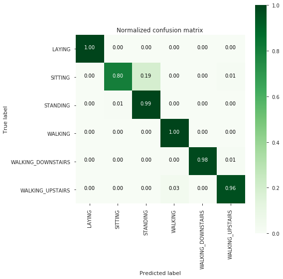
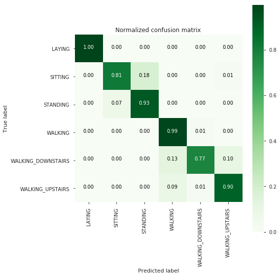
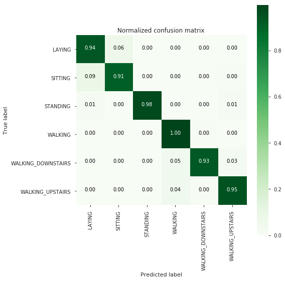
cm = metrics.confusion_matrix(y_test, np.argmax(y_pred, axis=1))
    # plot confusin matrix
plt.figure(figsize=(8,8))
plt.grid(b=False)
plot_confusion_matrix(cm, classes=labels, normalize=True, title='Normalized confusion matrix', cmap= plt.cm.Greens)
plt.show()
accuracy = metrics.accuracy_score(y_test, np.argmax(y_pred, axis=1))
# store accuracy in results
#results['accuracy'] = accuracy
print('---------------------')
print('|      Accuracy      |')
print('---------------------')
print('\n    {}\n\n'.format(accuracy))
---------------------
|      Accuracy      |
---------------------

    0.9501187648456056
from sklearn.metrics import classification_report , accuracy_score
print(classification_report(y_test, pred))
              precision    recall  f1-score   support

         0.0       0.91      0.94      0.92       532
         1.0       0.93      0.91      0.92       491
         2.0       1.00      0.98      0.99       537
         3.0       0.93      1.00      0.96       496
         4.0       0.99      0.93      0.96       420
         5.0       0.96      0.95      0.95       471

   micro avg       0.95      0.95      0.95      2947
   macro avg       0.95      0.95      0.95      2947
weighted avg       0.95      0.95      0.95      2947
Deep learning models is below the accuracy of basic ML model.
Next Steps
- Explore more on feature engineering
- Expand on deep learning models
- Productize the model, build an application and host on heroku /render
