Marketing Channel Attribution

1. Business Problem
We will be looking at Google Merchandise Store https://shop.googlemerchandisestore.com/ Customer who loves Google Products can buy tees, jackets and others swags from this website. In the website, Google Analytics tracks every event on the website. They do have multiple tocuh-points like Youtube, Google Ads, Referaal links etc.
Google has shared the data set (after normalization) in Google Big Query and we can use this data for Channel Attribution
1.1 Problem Statement
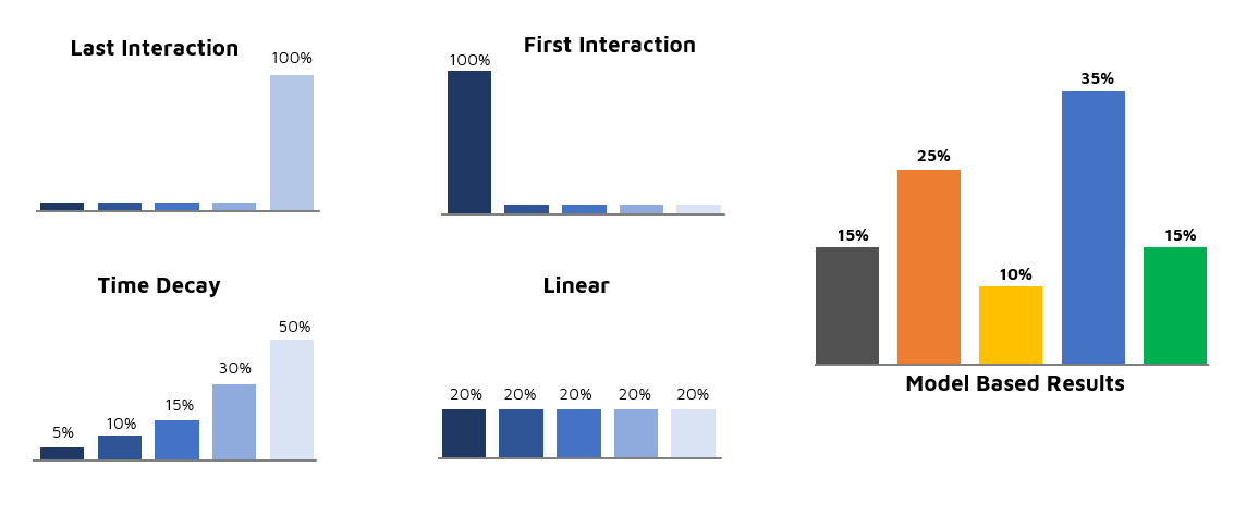
There are multiple Conversion Model that are widely used in Marketing domains. Below are some of them:
- First Interaction
- Last Interaction
- Time Decay Interaction
- Linear Interaction
We can use any of the Heuristic Models and mostly used in the industry is the Last Touch Model. The problem in the heuristic model is not to consider all the different channels from the application, which will hurt the overall conversion funnel.
 source: https://github.com/MatCyt/Markov-Chain
The solution in this case study is to capture the whole journey by using Markov Chain.
1.2 Data
We are fetching the daata from Google BigQuery in public data set freely avaible. Below is the query to fetch data:
# Databases
#library(bigrquery)
library(DBI)
#library(connections)
library(jsonlite)

# Core
library(tidyverse)
## -- Attaching packages --------------------------------------------------------------------------------------------- tidyverse 1.3.0 --
## v ggplot2 3.2.1     v purrr   0.3.3
## v tibble  2.1.3     v dplyr   0.8.4
## v tidyr   1.0.2     v stringr 1.4.0
## v readr   1.3.1     v forcats 0.4.0
## -- Conflicts ------------------------------------------------------------------------------------------------ tidyverse_conflicts() --
## x dplyr::filter()  masks stats::filter()
## x purrr::flatten() masks jsonlite::flatten()
## x dplyr::lag()     masks stats::lag()
library(tidyquant)
## Loading required package: lubridate
##
## Attaching package: 'lubridate'
## The following object is masked from 'package:base':
##
##     date
## Loading required package: PerformanceAnalytics
## Loading required package: xts
## Loading required package: zoo
##
## Attaching package: 'zoo'
## The following objects are masked from 'package:base':
##
##     as.Date, as.Date.numeric
##
## Attaching package: 'xts'
## The following objects are masked from 'package:dplyr':
##
##     first, last
##
## Attaching package: 'PerformanceAnalytics'
## The following object is masked from 'package:graphics':
##
##     legend
## Loading required package: quantmod
## Loading required package: TTR
## Version 0.4-0 included new data defaults. See ?getSymbols.
library(lubridate)
library(plotly)
##
## Attaching package: 'plotly'
## The following object is masked from 'package:ggplot2':
##
##     last_plot
## The following object is masked from 'package:stats':
##
##     filter
## The following object is masked from 'package:graphics':
##
##     layout
# dplyr helpers
library(dbplyr)
##
## Attaching package: 'dbplyr'
## The following objects are masked from 'package:dplyr':
##
##     ident, sql
# Attribution
library(ChannelAttribution)
query <- "
SELECT fullVisitorId, date, channelGrouping,
    trafficSource.source AS traffic_source,
    SUM ( totals.transactions ) AS total_transactions,
    SUM ( totals.totalTransactionRevenue ) AS total_transaction_revenue
FROM `bigquery-public-data.google_analytics_sample.ga_sessions_*`
GROUP BY fullVisitorId, date, channelGrouping, traffic_source;
"
1.3 Data Cleaning
In case, you don’thave bigQuery. I am sharing the bigQuery results in CSV file.
# Incase you don't need to run BigQuery; Use csv
query_tbl <- read_csv("data/bigquery_data.csv")
## Parsed with column specification:
## cols(
##   fullVisitorId = col_character(),
##   date = col_double(),
##   channelGrouping = col_character(),
##   traffic_source = col_character(),
##   total_transactions = col_double(),
##   total_transaction_revenue = col_double()
## )
query_tbl %>%
    count(channelGrouping, traffic_source, sort = TRUE)
## # A tibble: 287 x 3
##    channelGrouping traffic_source            n
##    <chr>           <chr>                 <int>
##  1 Organic Search  google               212125
##  2 Social          youtube.com          209881
##  3 Organic Search  (direct)             137501
##  4 Direct          (direct)             131037
##  5 Referral        (direct)              61801
##  6 Affiliates      Partners              15062
##  7 Referral        analytics.google.com  14328
##  8 Paid Search     google                11592
##  9 Paid Search     (direct)              10913
## 10 Display         dfa                    4935
## # ... with 277 more rows
query_tbl %>% count(channelGrouping, sort = TRUE)
## # A tibble: 8 x 2
##   channelGrouping      n
##   <chr>            <int>
## 1 Organic Search  356052
## 2 Social          222610
## 3 Direct          131037
## 4 Referral         94410
## 5 Paid Search      22506
## 6 Affiliates       15062
## 7 Display           5440
## 8 (Other)            107
query_tbl %>% count(traffic_source, sort = TRUE)
## # A tibble: 275 x 2
##    traffic_source            n
##    <chr>                 <int>
##  1 (direct)             341327
##  2 google               224182
##  3 youtube.com          209881
##  4 Partners              15069
##  5 analytics.google.com  14328
##  6 dfa                    4935
##  7 google.com             4443
##  8 baidu                  3287
##  9 m.facebook.com         3275
## 10 sites.google.com       2735
## # ... with 265 more rows
query_tbl %>% count(traffic_source, sort = TRUE) %>% glimpse()
## Observations: 275
## Variables: 2
## $ traffic_source <chr> "(direct)", "google", "youtube.com", "Partners"...
## $ n              <int> 341327, 224182, 209881, 15069, 14328, 4935, 444...
g <- query_tbl %>%

    # Cleaning
    mutate(traffic_source_clean = traffic_source %>%
               str_to_lower() %>%
               str_replace("\\.com", "") %>%
               str_replace("^m\\.", "")) %>%
    mutate(traffic_source_clean = case_when(
        str_detect(traffic_source_clean, "\\.google") ~ "google_product",
        str_detect(traffic_source_clean, "google\\.") ~ "google",
        str_detect(traffic_source_clean, "facebook") ~ "facebook",
        TRUE ~ traffic_source_clean
    )) %>%
    mutate(traffic_source_clean = traffic_source_clean %>%
               as_factor() %>%
               fct_lump(n = 3, other_level = "other_source")) %>%

    # Aggregating
    count(traffic_source_clean) %>%
    arrange(desc(n)) %>%
    mutate(traffic_source_clean = fct_reorder(traffic_source_clean, n)) %>%

    # Visualizing
    ggplot(aes(traffic_source_clean, n)) +
    geom_point(size = 5, color='darkblue') +
    coord_flip() +
    expand_limits(y = 0)


ggplotly(g)
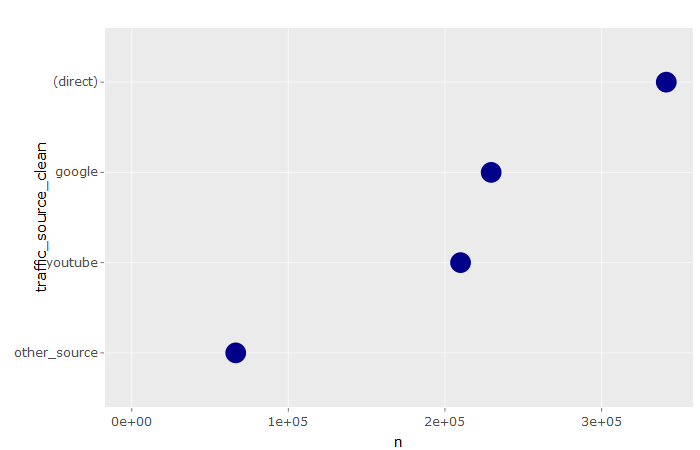
I have defined into four categories : Direct , Google , Youtube and others (all other sources are added in this group.)
# Apply Cleaning Steps
query_clean_tbl <- query_tbl %>%
    mutate(traffic_source_clean = traffic_source %>%
               str_to_lower() %>%
               str_replace("\\.com", "") %>%
               str_replace("^m\\.", "")) %>%
    mutate(traffic_source_clean = case_when(
        str_detect(traffic_source_clean, "\\.google") ~ "google_product",
        str_detect(traffic_source_clean, "google\\.") ~ "google",
        str_detect(traffic_source_clean, "facebook") ~ "facebook",
        TRUE ~ traffic_source_clean
    )) %>%
    mutate(traffic_source_clean = traffic_source_clean %>%
               as_factor() %>%
               fct_lump(n = 3, other_level = "other_source"))

query_clean_tbl %>% count(channelGrouping, traffic_source_clean, sort = TRUE)
## # A tibble: 19 x 3
##    channelGrouping traffic_source_clean      n
##    <chr>           <fct>                 <int>
##  1 Organic Search  google               212125
##  2 Social          youtube              209971
##  3 Organic Search  (direct)             137501
##  4 Direct          (direct)             131037
##  5 Referral        (direct)              61801
##  6 Referral        other_source          27276
##  7 Affiliates      other_source          15062
##  8 Social          other_source          12639
##  9 Paid Search     google                11592
## 10 Paid Search     (direct)              10913
## 11 Organic Search  other_source           6426
## 12 Referral        google                 5333
## 13 Display         other_source           4935
## 14 Display         google                  432
## 15 Display         (direct)                 73
## 16 (Other)         other_source             72
## 17 (Other)         google                   33
## 18 (Other)         (direct)                  2
## 19 Paid Search     other_source              1
2. Understand Value by Channel-Source - Attribution Analysis
# Attribution Analysis
channel_value_tbl <- query_clean_tbl %>%
    group_by(channelGrouping, traffic_source_clean) %>%
    summarize(
        n = n(),
        total_transactions = sum(as.numeric(total_transactions), na.rm = TRUE),
        total_transaction_revenue = sum(as.numeric(total_transaction_revenue), na.rm = TRUE) / 1e6
    ) %>%
    mutate(revenue_per_conversion = total_transaction_revenue / n) %>%
    ungroup() %>%
    arrange(desc(total_transaction_revenue))

channel_value_tbl
## # A tibble: 19 x 6
##    channelGrouping traffic_source_~      n total_transacti~
##    <chr>           <fct>             <int>            <dbl>
##  1 Referral        (direct)          61801             5348
##  2 Direct          (direct)         131037             2219
##  3 Organic Search  google           212125             2174
##  4 Organic Search  (direct)         137501             1360
##  5 Referral        other_source      27276              190
##  6 Paid Search     google            11592              248
##  7 Display         other_source       4935              132
##  8 Paid Search     (direct)          10913              231
##  9 Social          other_source      12639              120
## 10 Organic Search  other_source       6426               47
## 11 Display         google              432               18
## 12 Affiliates      other_source      15062                9
## 13 Referral        google             5333                5
## 14 Social          youtube          209971               11
## 15 Display         (direct)             73                2
## 16 (Other)         google               33                1
## 17 (Other)         (direct)              2                0
## 18 (Other)         other_source         72                0
## 19 Paid Search     other_source          1                0
## # ... with 2 more variables: total_transaction_revenue <dbl>,
## #   revenue_per_conversion <dbl>
3. Data Visulization
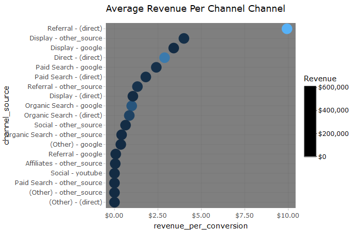
3.1 Visualize Average Revenue Per Channel
#Visualize Average Revenue Per Channel
g <- channel_value_tbl %>%

    # Make plot labels and sort order
    mutate(point_text = str_glue("Total Revenue: {scales::dollar(total_transaction_revenue)}
                                 Revenue Per Entry: {scales::dollar(revenue_per_conversion)}")) %>%
    mutate(channel_source = str_glue("{channelGrouping} - {traffic_source_clean}")) %>%
    mutate(channel_source = as_factor(channel_source) %>% fct_reorder(revenue_per_conversion)) %>%

    # Visualize
    ggplot(aes(channel_source, revenue_per_conversion)) +
    geom_point(aes(text = point_text, color = total_transaction_revenue), size = 5) +
    coord_flip() +
    scale_y_continuous(labels = scales::dollar_format()) +
    scale_color_continuous(labels = scales::dollar_format()) +
    labs(title = "Average Revenue Per Channel Channel", color = "Revenue") +
    theme_dark()
## Warning: Ignoring unknown aesthetics: text
ggplotly(g, tooltip = "text")
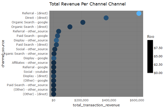
3.2 Visualize Total Revenue Per Channel
g <- channel_value_tbl %>%

    # Make plot labels and sort order
    mutate(point_text = str_glue("Total Revenue: {scales::dollar(total_transaction_revenue)}
                                 Revenue Per Entry: {scales::dollar(revenue_per_conversion)}")) %>%
    mutate(channel_source = str_glue("{channelGrouping} - {traffic_source_clean}")) %>%
    mutate(channel_source = as_factor(channel_source) %>% fct_reorder(total_transaction_revenue)) %>%

    # Visualize
    ggplot(aes(channel_source, total_transaction_revenue)) +
    geom_point(aes(text = point_text, color = revenue_per_conversion), size = 5) +
    coord_flip() +
    scale_y_continuous(labels = scales::dollar_format()) +
    scale_color_continuous(labels = scales::dollar_format()) +
    labs(title = "Total Revenue Per Channel Channel", color = "RPE") +
    theme_dark()
## Warning: Ignoring unknown aesthetics: text
ggplotly(g, tooltip = "text")
4. Data volume is in ~700K rows and used dtplyr (big data for data table)
query_dtplyr <- query_clean_tbl %>% dtplyr::lazy_dt()


visitor_date_channelgrouping_dtplyr <- query_dtplyr %>%

    # Fix date from BigQuery
    mutate(date = ymd(date)) %>%

    # Add Channel-Traffic Source Combo
    mutate(channel_source = str_c(channelGrouping, "-", traffic_source_clean)) %>%

    # Select Important columns
    select(fullVisitorId, date, channel_source, total_transactions, total_transaction_revenue) %>%

    # Fix revenue
    mutate(total_transaction_revenue = total_transaction_revenue / 1e6) %>%

    # Path Calculations
    group_by(fullVisitorId, date, channel_source) %>%
    mutate(total_transactions = sum(total_transactions, na.rm = TRUE)) %>%
    mutate(total_transaction_revenue = sum(total_transaction_revenue, na.rm = TRUE)) %>%
    arrange(date) %>%
    ungroup() %>%

    # Binary Conversion (Yes/No)
    mutate(total_transactions = ifelse(total_transactions > 0, 1, 0))

visitor_date_channelgrouping_tbl <- as_tibble(visitor_date_channelgrouping_dtplyr)
visitor_date_channelgrouping_tbl
## # A tibble: 847,224 x 5
##    fullVisitorId date       channel_source total_transacti~
##    <chr>         <date>     <chr>                     <dbl>
##  1 000722514342~ 2016-08-01 Direct-(direc~                0
##  2 001465993518~ 2016-08-01 Social-youtube                0
##  3 001569443280~ 2016-08-01 Direct-(direc~                0
##  4 001747219368~ 2016-08-01 Organic Searc~                0
##  5 001852659575~ 2016-08-01 Social-youtube                0
##  6 001998304603~ 2016-08-01 Direct-(direc~                0
##  7 002597793543~ 2016-08-01 Social-youtube                0
##  8 002855959112~ 2016-08-01 Direct-(direc~                0
##  9 003065339361~ 2016-08-01 Social-youtube                0
## 10 003651776577~ 2016-08-01 Social-youtube                0
## # ... with 847,214 more rows, and 1 more variable:
## #   total_transaction_revenue <dbl>
channel_path_dtplyr <- visitor_date_channelgrouping_dtplyr %>%

    group_by(fullVisitorId) %>%
    summarize(
        channel_path     = str_c(channel_source, collapse = " > "),
        conversion_total = sum(total_transactions),
        conversion_null  = sum(total_transactions == 0),
        conversion_value = sum(total_transaction_revenue),
        n_channel_path   = n()
    ) %>%
    ungroup()

channel_path_tbl <- channel_path_dtplyr %>% as_tibble()

# Longest Channel Path?
channel_path_tbl %>% arrange(desc(n_channel_path))
## # A tibble: 714,167 x 6
##    fullVisitorId channel_path conversion_total conversion_null
##    <chr>         <chr>                   <dbl>           <int>
##  1 195745897629~ Organic Sea~               14             132
##  2 360847519334~ Paid Search~                1             130
##  3 072031119776~ Social-othe~                0             119
##  4 082483972611~ Organic Sea~                0             117
##  5 403807668303~ Organic Sea~                0             110
##  6 185674914791~ Organic Sea~                0             104
##  7 326983486538~ Direct-(dir~                1              87
##  8 601877531773~ Direct-(dir~                0              83
##  9 980127621496~ Organic Sea~                0              83
## 10 369423402852~ Direct-(dir~                1              73
## # ... with 714,157 more rows, and 2 more variables:
## #   conversion_value <dbl>, n_channel_path <int>
# Most Path Conversions?
channel_path_tbl %>% arrange(desc(conversion_total))
## # A tibble: 714,167 x 6
##    fullVisitorId channel_path conversion_total conversion_null
##    <chr>         <chr>                   <dbl>           <int>
##  1 781314996140~ Direct-(dir~               28              22
##  2 498436650112~ Direct-(dir~               16               5
##  3 240252719973~ Direct-(dir~               15              13
##  4 195745897629~ Organic Sea~               14             132
##  5 676073240225~ Referral-(d~               14              15
##  6 060891519773~ Referral-(d~               13               2
##  7 731124288608~ Direct-(dir~               12              10
##  8 207416433864~ Direct-(dir~               11               8
##  9 819787964379~ Organic Sea~               10              27
## 10 908913239224~ Direct-(dir~               10               9
## # ... with 714,157 more rows, and 2 more variables:
## #   conversion_value <dbl>, n_channel_path <int>
5. CHANNEL ATTRIBUTION MODELING
5.1 Plotting Utility
plot_attribution <- function(data, title = "Attribution Model", interactive = TRUE) {
    g <- data %>%
        pivot_longer(
            cols = -channel_name,
            names_to  = "conversion_type",
            values_to = "conversion_value"
        ) %>%
        mutate(channel_name = as_factor(channel_name) %>% fct_reorder(conversion_value)) %>%

        ggplot(aes(channel_name, conversion_value, fill = conversion_type)) +
        geom_col(position = "dodge") +
        theme_tq() +
        scale_fill_tq() +
        coord_flip() +
        labs(title = title)

    if (interactive) return(ggplotly(g))
    else return(g)
}
5.2 Heurisitic Models
channel_path_heuristic_model <- channel_path_tbl %>%
    heuristic_models(
        var_path = "channel_path",
        var_conv = "conversion_total",
        var_value = "conversion_value",
        sep = ">"
    )
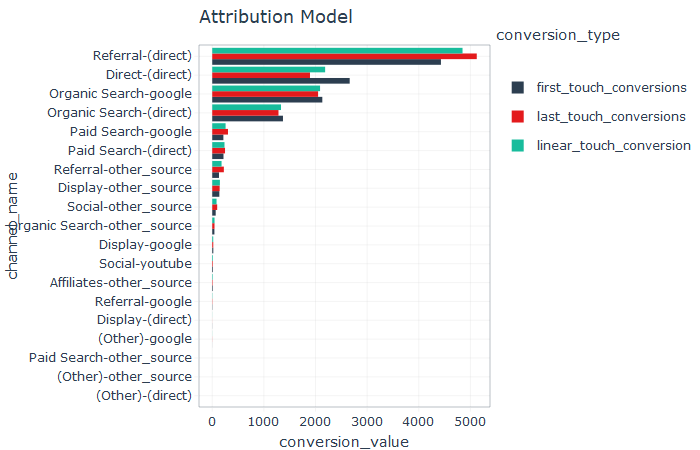
5.3 Data Visualization
# Conversion Count
channel_path_heuristic_model %>%
    select_at(vars(channel_name, matches("conversions"))) %>%
    plot_attribution()
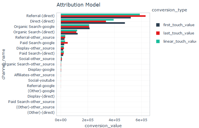
# Conversion Value
channel_path_heuristic_model %>%
    select_at(vars(channel_name, matches("value"))) %>%
    plot_attribution()
6 Markov Chain
markov_model <- channel_path_tbl %>%
    markov_model_mp(
        var_path = "channel_path",
        var_conv = "conversion_total",
        var_value = "conversion_value",
        sep = ">",
        order = 3,
        nfold = 10,
        seed = 123
    )
## Number of simulations: 100000 - Convergence reached: 0.028860
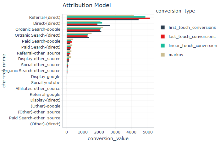
# Conversion Count
markov_model %>%
    select(-total_conversion_value) %>%
    rename(markov = total_conversion) %>%
    left_join(
        channel_path_heuristic_model %>%
            select_at(vars(channel_name, matches("conversions")))
    ) %>%
    plot_attribution()
## Joining, by = "channel_name"
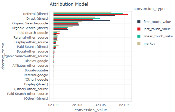
# Value
markov_model %>%
    select(-total_conversion) %>%
    rename(markov = total_conversion_value) %>%
    left_join(
        channel_path_heuristic_model %>%
            select_at(vars(channel_name, matches("value")))
    ) %>%
    plot_attribution()
## Joining, by = "channel_name"
7. Conclusion
It was a great introdction to Google Merchandise of Marketing Attribution with use of heuristics and Markov Chain.
8. Next Steps
- We will the Split Paths by Transactions
- Data Visualization of paths
- Use of Machine Learning - http://www0.cs.ucl.ac.uk/staff/w.zhang/rtb-papers/data-conv-att.pdf
